02 Jun 2022
There are some rare events in your life which you know will be the turning point for what comes ahead. ICRA 2022 was one of those for me.
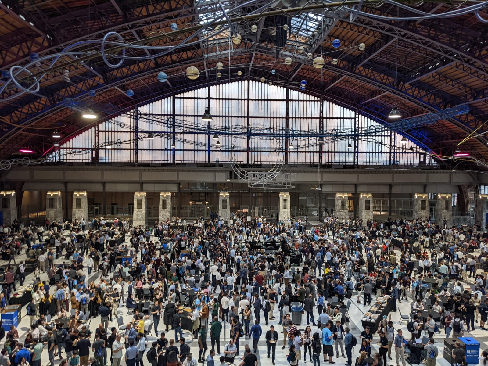
ICRA, the International Conference for Robotics and Automation is the largest robotics conference in the world and witnesses thousands of attendees from dozens of countries. This year's ICRA was particularly special as it was the first time ICRA was held in person since ICRA 2019 in Montreal. It was special to me too as it was held in Philadelphia right after my graduation ceremony from the University of Pennsylvania. The timing could not be better and I am delighted that NVIDIA fully sponsored me to attend the whole conference comprising of two days of workshops and three days of exhibits, technical talks, and poster presentations. While this isn't my first international conference, it is my first academic conference.
There was little reason to doubt the scale of the conference when I saw the length of the line for registration at 830am on the opening day. It took me a good 5 minutes to walk to the end of the line, which wrapped around the ground floor of the enormous atrium of the Pennsylvania Convention Center. Standing in line gave me a good chance to survey the crowd, comprising of a mix of industry professionals and PhD students. I guess the professors and post-docs had the good sense to collect their badge from the convention center the previous day since I didn't see any waiting in line. On reaching the front of the line, I collected my ICRA kit containing my conference badge, an ICRA branded bag, three adorable stickers for my badge to indicate whether I preferred to elbow bump, shake hands, or hug, and (what would become a theme for the conference) an ICRA T-shirt!
I attended the workshops on novel perception techniques and autonomous driving. I also got a sneak peek of the company exhibition booths on the second level of the convention center. Apart from being a great place to meet researchers, I learned ICRA also serves as a recruiting event for several startups and more established robotics companies such as Skydio, Dyson, Motional, and Tesla. Over the following days, I amassed enough company swag to cover my clothing needs for the entire the conference. Had I known better, I would have probably packed a little lighter.
The day ended with a huge networking dinner in the ballroom of the convention center. Over dinner I was pleasantly surprised to meet old friends who I didn't even know were attending and even one of my TA's at UPenn who had successfully raised millions of dollars in funding for his autonomous lawnmower startup, Novabot!

The autonomously lawn mowing Novabot, developed by my CIS581 TA Yulai Weng!
It had been such a long time since anyone had attended an event of this size and it was clear that everyone was relishing the opportunity to socialize and geek out. For someone who wouldn't normally walk up and talk up to people unsolicitedly, I found myself really enjoying the process of introducing myself and learning about what other people were working on.
Networking dinner at the end of day 1! Where's Waldo?
The next three days formed the main part of the conference with technical presentations, company exhibitions, and boozy recruitment parties. This year's ICRA adopted a hybrid model for the paper presentations. Compared to the first ICRA in 1985 which had one track with each 25 minute presentations, ICRA in 2022 had 22 parallel tracks with 5 minute lightning talks in the morning and afternoon. I felt 5 minutes was barely enough time to grasp the keywords of the paper, especially if it was in a field which I hadn't worked in before. Fortunately, the lightning talks were followed by in-depth poster presentations where you can walk up and ask the authors questions about their work. I found great value in the poster presentations and ended up learning a lot by talking to the authors.
As an aside about the hybrid model of presentations, some authors chose to present using a 5 minute video of them speaking over their slides and answering questions over Zoom. It was somewhat ironical that we had gathered from thousands of miles away only to watch a video together.

My school friend's, Aditya Arun's, poster presentation!
I also loved attending the company exhibition booths in between the paper presentations, especially those where engineers from the companies came to describe what they were working on. Based on the booths, my impression of the robotics industry is that it is dominated by a new wave of software companies either 1) leveraging existing hardware (particularly UAVs and service bots) for new applications or 2) providing tools for other robotics companies. Companies like Skydio, Shield AI, and OhmniLabs fall into the first category whereas companies like Foxglove and Tangram Vision fall in the second. What was less common was companies providing hardware (such as sensors and motors) to companies in the first category such as Ouster and DirectDrive motors. The exhibitions piqued my curiosity for how these startups discover a market niche and create products to fill said niches.
The second day of the conference ended on a high with the Skydio recruitment party at a bar in Philadelphia's Chinatown called bar.ly. Over beer, I chatted with some European post-docs and PhD students who had a hand in designing the Mars helicopter, Ingenuity. Ingenuity has to contend with some of the most outlandish conditions any robot has experienced and has to sustain aerial flight in an atmosphere 1% of the thickness of Earth's. Roughly speaking, that equates to flying a drone at an altitude of 100,000 feet above Earth's surface (albeit in lower gravity). I also learned that robot localization is much more challenging on Mars, for the planet's lack of a magnetic field makes magnetometers useless and for the time being at least, the planet is bereft of a GPS/GNSS network. Surprisingly, that makes visual inertial odometry (VIO) the most effective way to localize Martian robots. However, Mars's surface is devoid of significant visual features which VIO algorithms heavily rely on. To this end, the VIO algorithm for Ingenuity was tested on deserts on Earth which lack significant visual features the way the Martian surface does. As Ingenuity is experimental hardware, it can use the consumer-grade Snapdragon 801 for its flight computer whereas other space robots use much slower, radiation hardened processors for better reliability.
ICRA also had some great keynote talks with Julie Shah opening Day 3 with a talk about what the future of robots and humans working together might look like. It never occurred to me that safety for the humans and task efficiency for the robots working with them could be conflicting goals. Research in this area deals with designing ways robots can better predict the actions of humans and how they can offer social cues when working alongside them. Another challenge is making complex machines like robots easy to train and maintain for operators.

Me at the morning keynote session!
In a more formal setting than the discussions I had about the same topic the previous night, the afternoon keynote talk was by Prof. Vandi Verma at NASA, who spoke about the challenges of space robotics and the development of Ingenuity. I learned that the only picture of the Perseverance rover and Ingenuity in the same frame was shot with painstaking composition and caution, since the robotic arm carrying the camera has to be aligned correctly with the rover's other instruments. Who would've thought that something as simple as taking a picture involves hours of simulations back at NASA?
Ingenuity and Perseverance in the same frame! Hours of planning went into this shot.
I also watched the semifinals and finals of the F1Tenth racing competition in which teams race self-driving 1:10 scale cars on an indoor track. I have particularly fond (and painful) memories of hacking together our own autonomously driven racecar in my second semester at UPenn. It was super impressive to see how far the project had come along with all the top team's approaches having robust controllers, overtaking maneuvers, and even blocking maneuvers to avoid overtakes. I daresay that it's even better than watching the 'real' F1 races! UPenn's very own Team ScatterBrain brought the trophy home in a head to head final race with Dzik from the Czech Republic.
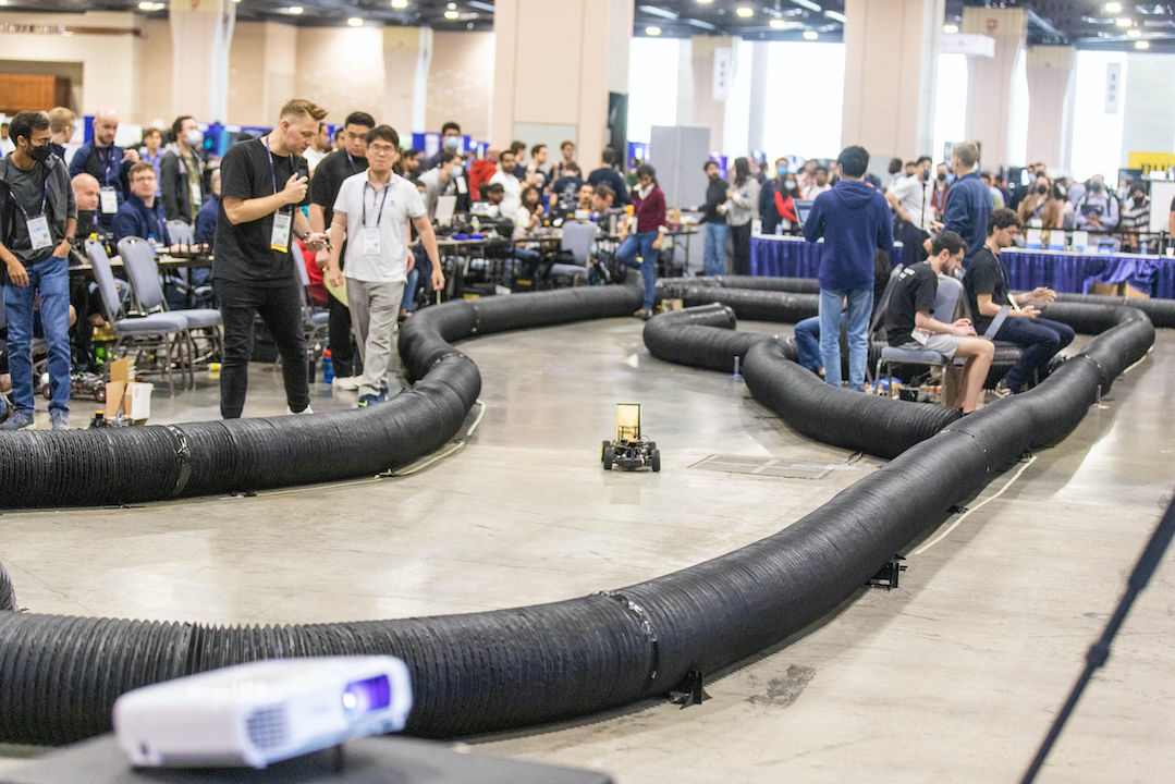
Johannes Betz commenting on the F1/10 races!
The day ended with a banquet dinner in the terrace of the convention hall with speeches from Prof. Vijay Kumar at UPenn and Spot from Boston Dynamics raising a toast to all robots (and humans behind them)!
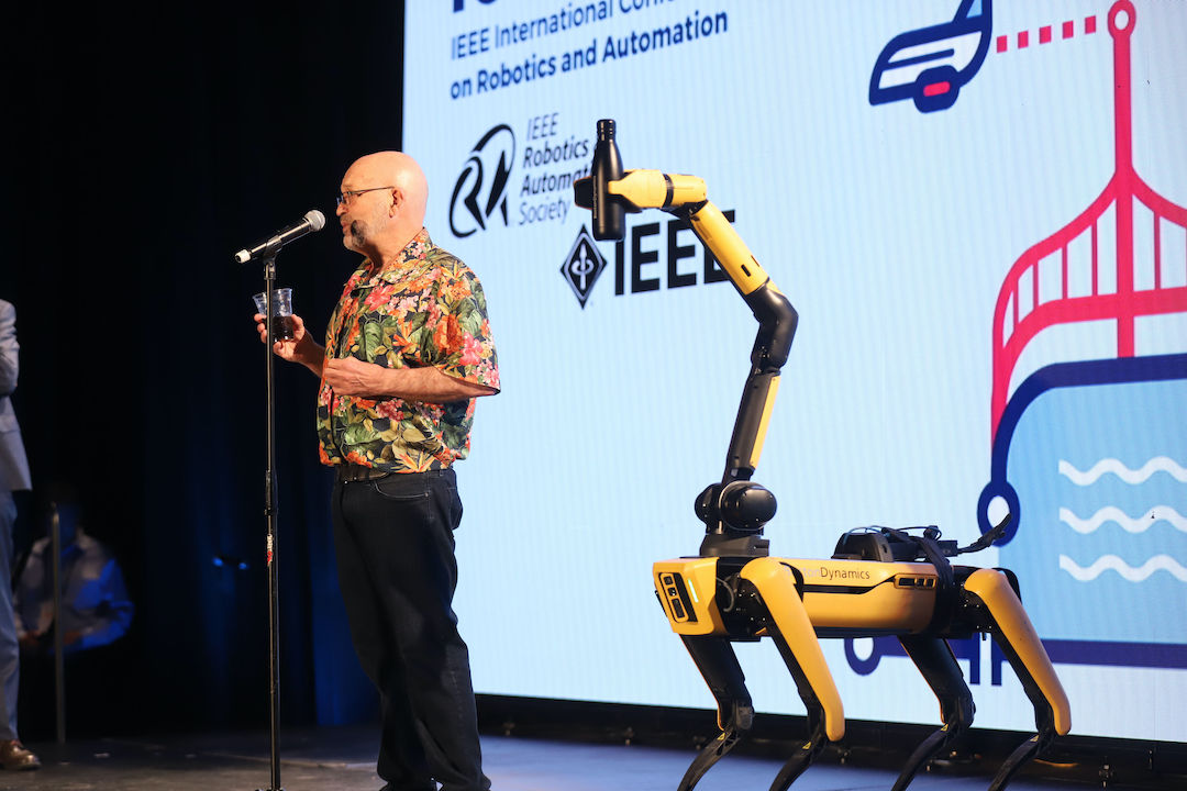
Spot raising a toast to all the robots out there!
The penultimate day of the conference had technical presentations on topics which I work closely on at work - autonomous vehicle navigation and motion planning. Some of the presentations which stood out to me were 1) StopNet for whole scene prediction modelling from Waymo, 2) trajectory generation to maximize information gain in the presence of occlusions and 3) PredictionNet from our very own prediction team at NVIDIA. It was interesting to compare the differences in StopNet and PredictionNet, for the former is a sophisticated prediction model which shows what is possible when you have significant computational resources (more than 1TFLOP per inference!) to throw at the problem whereas the latter is an efficient prediction model which is designed to run in a few milliseconds on the NVIDIA Drive AGX platform. I also came away with the impression that its genuinely difficult to produce good quality research for autonomous vehicles at the university level. Several papers only had results in simulation which is hardly sufficient for demonstrating the validity of an approach. An end-to-end model which goes directly from camera pixel values to steering wheel torques may look impressive when demoed in CARLA, but it seldom holds water when implemented in a real vehicle. For better or for worse, the autonomous vehicles testing pipeline requires trained test drivers, testing tracks, expensive sensors, and of course, cars, which are expensive to retrofit with sensors and specialized hardware. This is very capital intensive and out of the reach for all but a few universities. With some bias, I am of the opinion that for this reason, most of the useful progress in the field will be led by the industry. On that note, the conference session ended with a panel discussion on the future of the AV industry with research leads from Tesla, Motional, Zoox, NVIDIA, Toyota Research International, Waymo, and Qualcomm chiming in. And as on brand for this conference, the night ended in more revelry with Zoox footing the bill for drinks and finger food at the Graffiti Bar in Philadelphia's Center City.

Robots (and exoskeletons)!
With the technical talks and exhibition booths wrapped up on Thursday, the final day of the conference felt subdued compared to the ones before it, though this is in no small part due to the action of the last handful of days catching up to me. I flitted between workshop rooms to learn more about the latest in neural geometry based motion planning (think NeRFs) and autonomous driving. Lunch was followed by one of my favorite events at ICRA in recent years - the robotics debates. I attended the debate on 'The investment and involvement of industry giants in robotics research in academia is positive'. At the outset, I felt it would be hard to argue against this topic and voted 'Yes' in the pre-debate polls. I was proven wrong by Prof. Ankur Mehta who made an excellent case for how in some ways, the funding offered by huge companies can create perverse incentives for academic research labs to pursue avenues of research which are more oriented towards creating profit for big tech companies. The relation between industry funding and universities is not always as synergistic as it may seem. Personally, I still feel that the industry and universities have benefitted from each other's goals, but I am more on the fence about if it's always a good thing. Academia and the robotics industry will always be competing for the best minds to join as PhDs or postdocs in the former's case and as skilled engineers in the latter's. What kind of systemic change is required so both can benefit without being at odds with each other?
At this point, my brain had pretty much checked out of ICRA and I attended the final workshop on motion planning under uncertainty, but couldn't do much more than passively listen.
Despite being physically and mentally tired on the last day, I left the conference feeling very inspired. It's hard not to be when you get time to interact face-to-face with people who are so venerated in the robotics community. There is something special about the energy of having thousands of people with the same interests together in a single room and I now understand why these conferences are such a big deal. It was a humbling experience too - for it showed me that there was so much I didn't know in the very field I spent two years getting a masters degree in. I am bullish for the future prospects of robotics as ICRA has showed me that academic and industrial interest in solving the biggest open problems of robotics is at an all time high. People are seriously thinking about the inevitable ways in which our society will change once robotics become much more commonplace. And finally, automation could unlock huge markets of opportunity which didn't exist before.
On a more personal note, I feel like my trip to the East coast this time has done me a world of good. Last year, I had written about how much I was looking forward to moving out of Philadelphia, but this time, I realized how much I had missed the city. Now that it's summer, Center City and its numerous parks are filled with people and there is much joy to be found on the streets. The city has a charm which hasn't been lost on me at all. I long for the spontaneity of urban life when living in the dull suburban sprawl of the South Bay. I feel like the 3000 miles of distance has given me a new perspective to reflect on life since moving to California. I have realized that despite having great friends nearby and a job I look forward to everyday, it all feels strangely devoid of contentment - something I say knowing full well that it comes from a position of immense privilege. That said, the general feeling of discontent is something echoed by the few with whom I've dared to broach the topic with as well. This is where I feel the conference was could be a turning point. ICRA has shown me that I feel at my best when talking to people and thinking about robotics outside of work. This is something I which I want to channelize in my weekdays as well, for I feel it's all to easy to get stuck in a loop of expending one's mental faculties at work and not leaving room for creative pursuits. There is so, so much magic left in robotics that I simply can't hope to cover all of it. In a way, it's a beautiful thing to be in a field where everyone can pick their own set of skills to be unique.
08 Jan 2022
Model Predictive Control (MPC) is an incredibly powerful technique for computer aided control of a system. MPC is now used in areas such as aircraft autopilot, traction control in cars, and even HVAC systems to reduce energy costs. In robotics, MPC plays an important role in trajectory generation and path following applications. That said, MPC found its roots in the 1980s in an entirely different type of industry - chemical and oil refinery. Back in those days, compute power was scarce and expensive. By applying an MPC control scheme to the plant's control systems, operators could save a lot of money which more than justified the cost of using expensive computers. Over time, with increases in compute power and efficiency, it became feasible to run optimization routines for realtime applications.
Before learning about MPC, I only knew about PID control and like PID, MPC is also a closed loop control scheme where the input chosen at a particular time depends on the current state of the system.
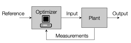 Block diagram of MPC, stolen from Prof. Morari's lecture slides
While PID can work reasonably well without any knowledge of the system we're controlling, MPC needs a model of the system we are working with. The benefit of using MPC is that we can obtain an optimal series of inputs if we implement our controller correctly. We can even define what optimal means depending on our application. For instance, for an autonomous drone, an optimal trajectory may be one that minimizes the energy used. On the other hand, for a robotic manipulator, we might want to optimize for minimizing the deviation from a planned trajectory.
One of my favorite parts of MPC is that the theory delves into a number of diverse topics such as control theory, convex optimization, and even computational geometry. With this blog post, I want to give an introduction to MPC and some of its associated concepts.
Discrete Systems
Most practical MPC implementations work with linear, discrete time systems. As the name implies, these are represented with a linear equation as:
\[x_{t+1}=Ax_t+Bu_t\]
where $x_t$ represents the state of the system, $A$ is the state transition matrix, $B$ is the input matrix, and $u_t$ is the input. $\Delta_t$ refers to the time discretization of our system. As an example, if we have a drone with a flight computer which can control the motors and sense the drone's state at 10Hz, we would want to set $\Delta_t$ to 0.1s. Our choice of state $x_t$ in this case is vector representing roll, pitch, and yaw, and our control input $u_t$ can be a vector of throttle inputs to the drone's motors.
What the above equation is telling us is that given the current state and control input of our system, we can calculate the state of the system at the next timestep. This is the model of the system which helps us predict the future states in our control scheme.
This simple equation is surprisingly powerful and it can be used to represent many different types of control systems. We can even represent systems with non-linear functions (such as sine, cosine, etc.) in their state transition matrix by linearizing the function at each timestep about an operating point.
This explanation is incomplete without an example and I suggest taking a look here for one. Although the system in the example is a continuous time system, discrete time system equations (mostly!) work the same way. The main difference between the continuous system in the example and discrete time systems we are dealing with here is that continuous systems calculate the rate of the system, whereas discrete time systems calculate the next state given the current state.
Cost Function
There are many ways to formulate an MPC problem, but the one we're going to look at here is picking a series of $n$ control inputs $u_0, u_1,..,u_{n-1}$ to stabilize a system to equilibrium. This means that by applying these $n$ inputs one after the other, we should be able to make the state of the system result in all zeroes at the end.
To use an optimizer based approach for finding an optimal solution, we need a cost function to evaluate the current state. We may also want to be economical with the amount of input applied, so we can assign a cost for the input applied too.
The choice of cost function is based on our problem and there are often different options we can choose to minimize. That said, we would ideally want to pick a cost function which can be optimized easily with the optimization tools we have at hand. For many practical problems, a quadratic cost function is a great choice. This cost function is convex, which guarantees we will find a globally optimal solution if it exists! Moreover, there are open-source implementations of quadratic program solvers such as OSQP. MATLAB's quadprog works well for these problems too. With a quadratic cost function, and a constraint on our input* our cost may look like this for a single timestep:
\[x_t^TQx_t+u_t^TRu_t\]
In this we can see that $x_t^TQx_t$ is the cost of the state of the system. If $Q$ is positive definite, any non-zero state will have a positive cost. If the system is at equilibrium, the cost will be 0. We can also intuitively see from the equation that if the L2 norm of the state is larger, the cost of the state will be roughly larger as well. Similarly, the term $u_t^TRu_t$ assigns a higher cost for larger inputs.
We can pick a diagonal matrix $Q\geq0$, and scalar $R\gt0$ so our cost is positive if we're not at equilibrium. We also enforce $\pm u \leq 1$ for the input constraint.
First, let's (quite charitably) assume we have all the time in the world to stabilize our system. We can then keep picking inputs at each timestep until our system is stable. If we have infinite time, we need to pick a series of infinite inputs! So our overall cost for the entire series ends up looking like:
\[\sum^{\infty}_{t=0} x_t^TQx_t+u_t^TRu_t\]
Fortunately, the above sum is not actually infinite, as once we have driven the system to stability, we don't need to apply any more inputs if the system is stabilizable. All the terms in the above are known because of the recurrence relation we know from the model of the system. But its clearly infeasible to optimize over an infinite series of states and inputs, and this brings us to the next innovation in MPC.
*If we didn't have any constraints in this optimization problem, an LQR controller would've given us a closed form optimal solution by solving the Discrete Algebraic Ricatti Equation (DARE, isn't this a cool acronym?).
Finite Horizon
Based on sound mathematical arguments which I won't discuss here, we don't actually need to compute the solution for infinite states. Instead, we can set a time horizon of a finite number of future $N$ states. This reduces our optimization problem to:
\[\text{minimize } \sum^{N-1}_{t=0} x_t^TQx_t+u_t^TRu_t+x_N^TPx_N\\
\text{subject to } x_{t+1}=Ax_t+Bu_t \text{ and} \pm u \leq 1\]
The last term $x_N^TPx_N$ tacked on to the summation is terminal cost which is our estimate for what the remaining cost till infinity will be. This is key here, we are trying to approximate an infinite sum with a reasonable guess for what the infinite sum should be. The choice of the positive definite matrix $P$ is also upto us, but it typically has larger eigenvalues than $Q$. The terminal state also needs to belong to a terminal set which can be calculated using other techniques based on our model.
We will get inputs $u_1,u_2,…,u_{N-1}$ from plugging the above summation into our optimizer of choice. Now, we come to the control part of MPC! We will only use the first input and discard the rest! This sounded wasteful to me when I was first learning about MPC, but the reasoning behind this is that inputs after $u_1$ are calculated based on future states based on our assumed model of the system. In other words, the input $u_2$ we will apply after applying $u_1$ assumes that we would have perfectly reached $x_2=Ax_1+Bu_1$. However, this is based on our model for the system's dynamics. In the real world, there will be differences in the state we get after applying $u_1$ because of noise, potential linearization error, state estimation error, and errors in our assumption of what the system's model is to begin with. From a closed loop control perspective, it also makes more sense to only apply the input corresponding to our current state.
Once we have applied $u_1$, we repeat the optimization procedure after measuring our state after applying this input. Just as with the other parameters we have discussed before, the length of the finite time horizon depends on our problem. Too short and it won't be optimizing over enough states to give us an optimal solution. Too large and our quadratic program might take too long for solve for the hardware we have at hand. On that note, we would ideally want the upper bound of the MPC procedure's runtime to be the length of one timestep $\Delta_t$. That way, we will have the solution ready before we apply the next input.
Matrix Construction
Quadratic program solvers take a cost function in the form of a single matrix $H$, which is internally used to evaluate $X^THX$ with (optional) constraints on the states. This means we have to rewrite our summation above in the form of a single vector representing all the variables in our optimization. There are two main ways we can do this:
- QP by substitution: replace all the states $x_1…x_n$ by inputs by applying the substitution $x_{t+1}=Ax_t+Bu_t$ everywhere. Optimize only over the inputs.
- QP without substitution: use the equation $x_{t+1}=Ax_t+Bu_t$ as an equality constraint and optimize over both states and inputs. This increases our optimization variables, but this method is actually more computationally efficient than using substitution.
More about these methods can be found from slide 33 onwards here.
While out of scope of this article, there are even ways to find closed form solutions to the MPC problem! A closed form solution can save us from running a computationally intensive optimization routine every timestep. This method deserves an article of its own and it has many benefits in real world applications. We can use this to compute the closed form solution offline and then evaluate the solution using these equations on the target hardware which may not be powerful enough to run the optimization procedure in real time.
To Sum Up
MPC is a valuable tool and we have several 'hyperparameters' we can play with like the cost matrices, length of time horizon, and the cost function itself. Finding a good set of parameters requires trial and error based on how our system actually behaves on running on our controller. This post only scratches the surface of MPC, so if you want to learn more about predictive control in all its glory, check out the links in the references section!
References
14 Sep 2021
I originally wrote a rough draft of this post on my flight from Philadelphia to California on 17 June 2021, but never got around to publishing it until recently.
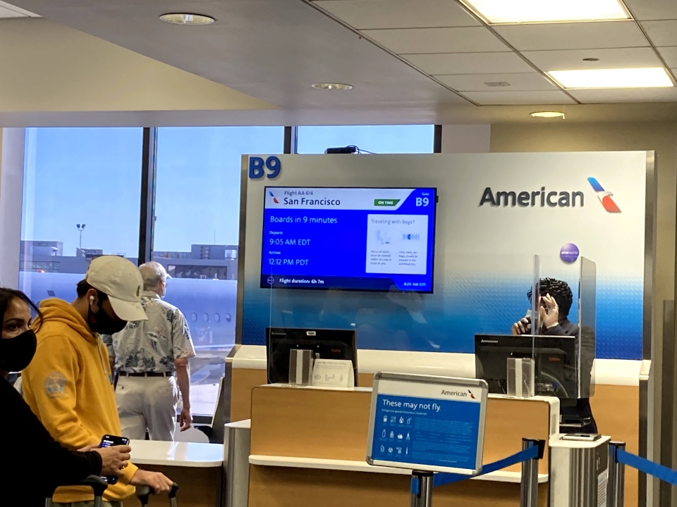 Waiting in anticipation of my flight from Philadelphia to California!
It's taken me a lot longer to write this post than I wanted to. It's harder for me to reflect on my experience as a ROBO MS student at UPenn as it typically would be as more than half of it was in a time of untold uncertainty. The pandemic uprooted campus life entirely and and it's not possible for me to view the masters experience without it.
Compared to the three online semesters I've had, I would unequivocally say that my first semester was the best one. I never took a single class for granted. There were several moments in my first semester where I used to pinch myself when walking to class on Locust Walk, thinking to myself that I had finally arrived at a utopia where I could study just what I wanted to and had all the resources to do anything I could imagine. It was the realization of a dream I wrote about back in my first year of undergrad. But midway through the second semester, the image of the utopia I had in mind was shattered once it became clear that COVID would become a major factor in all the decisions I would have to make to salvage whatever I could from the degree - from the courses I could take to the labs I could choose to work with. There was a lot of variation in my workload during the online semesters, for I worked part-time for a lab during the summer of 2020, worked full-time for a professor's startup while studying part-time in my third semester, and studied full-time in my final semester.
But now, on the other side of the MS degree, I am in a position I would have been thrilled to be in two years ago. I am very grateful that I was able to graduate with a GPA I can be proud of and with an exciting career in robotics at NVIDIA's autonomous vehicles team. The road to finishing the masters degree was long and difficult, and at some points in 2020, it felt like there wasn't a road to go on at all. Despite that, things have fallen into place for me remarkably well. And now, writing this blog post on my first business trip, I feel like I have made it, though not in a way I could have expected.
I read an article last year in the early days of COVID which said that the final stage of the grieving process is looking for meaning during times of hardships and tragedy. In a time when COVID has taken something from everyone, the only thing that one can gain is some of justification of all the struggles of a very different year. Personally, it has shown me what really matters and what things are worth worrying about. From as long as I can remember, I have been obsessively worried about things going wrong despite every indication that they weren't. It wasn't always a bad thing because the image of failure in my head pushed me to work harder. But when COVID became an emergency and the health of people I cared about became a primary issue, it made the problems I faced during my first semester seem a lot less significant. I still shudder when I think back to the long periods of isolation back in the summer of 2020. It was a rude awakening that I should have tried building a better social life before the pandemic, because there was no way to establish one with the pandemic raging. I was very fortunate that I had a very supportive friends circle that I could reach out to whenever I needed a pep talk during that time.
I have started seeing changes in myself as well. On the positive side, I am much more ready to go out and interact with new people than I ever have been. In some ways, it's just the phase I want going into a new city. On the other hand, the solitude I enjoyed so much in 2019 now makes me uncomfortable and it reminds me of the long periods of sitting alone in 2020. A side effect of this is that I don't want to tinker or work on side projects as much. That was also the case during the two years of masters' as well since my coursework more than whetted my appetite for wanting cool things to work on.
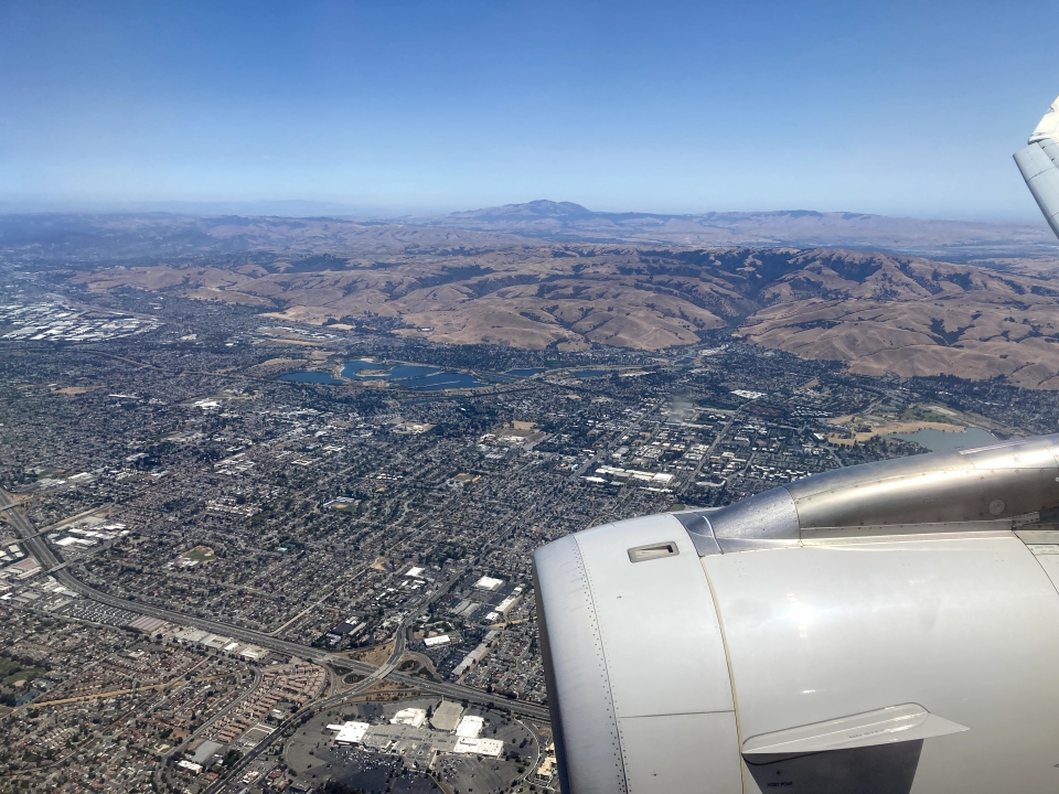 Deja vu and excitement on seeing the Bay Area after years
I feel like there's tremendous opportunity even before starting my new job at NVIDIA. I was exhilarated on getting the offer for this job nearly a year before the joining date. It completely turned my terrible summer around as the security of having a solid job offer in hand can not be understated when everything else seemed so uncertain last year. Though I have had some memorable internship projects in the past, I have never worked at a 'real' company before, so I am excited to see how an engineering team works at such a large organization. I feel like the last two years have been a build-up for this job and I'm really looking forward to actually applying what I learned during my degree to a business application. Most of my robotics coursework was either completely theoretical or only practically implemented in simulation. My brief experience of deploying robotics algorithms on a physical robot showed me that it is almost always is a frustrating experience. It is a necessary rite of passage to move out of simulation land for any robotics engineer and if all goes well, I should have plenty of opportunities to do that in this role.
I am also looking forward to moving out of Philadelphia. I've made many great memories during my two years in the city, but living in West Philadelphia was never a comfortable experience. Besides the general sense of urban decay to the north of Market and west of 40th St, I absolutely loathed the five months of freezing weather and early sunsets forcing everyone inside. From whatever I've heard about the Bay Area, I feel like life there will suit me much more than any other place I've lived before. I expect there'll be a learning curve of getting used to this new phase of life, but I don't expect it to be as steep as the ones I've had in the past when moving to a new place.
11 Sep 2021
The summer of 2021 was glorious and one of my first trips this summer was a very memorable visit to the Cherry Springs State Park, located in the middle of rural Pennsylvania. Situated on top of a mountain and hundreds of miles away from any major city, Cherry Springs is a world famous stargazing spot frequented by many hobbyist and professional astronomers with camping grounds booked for months on end. On a clear night one might expect to see hundreds (if not thousands) of stars, comets, Messier objects, and even a glimpse of the Milky Way galaxy. Unfortunately, clear nights are hard to come by at Cherry Springs with only 80-90 clear nights in a year. Coupled with the fact that the best time to go is during a new moon, it can be tricky to plan a trip to the park more than a few nights in advance. I highly recommend checking out the sky conditions for stargazing at ClearDarkSky. Ideally it should be as dark as possible with minimal cloud cover.
Cherry Springs Park has multiple astronomy sites, but unless you book in advance, you will most likely end up going to the Night Sky Public Viewing area near the campgrounds. The Public Viewing area is a massive field where one can setup their telescopes and cameras.
Our trip to Cherry Springs Park started from Philadelphia and was only really set in motion at the last minute after finding a rental car and a party of seven people who would didn't mind driving out 500 miles to spend the night outside. Our drive to CSP took us through several towns and villages once we got off the highway. The last leg of the trip is particularly challenging with winding mountain roads and several deer prancing across. As expected of a mountain road near a stargazing site, there are no streetlights and the surroundings are pitch dark. We had to cautiously make our way up the mountain with the car's high-beams on the whole time. Thankfully, the drive was uneventful and we reached the park at about 1130pm, giving us several hours before dawn.
On stepping out of the car, I felt the frigid mountain air on my face. While it was a balmy 25C in Philadelphia, the temperature on top of the mountain hovered around 0C. I was silently hoping that the sleeping bag that I brought with me for the trip would be up to the task of protecting me from the elements for the night. I took a quick glimpse of the night sky, and even though my eyes were still adjusting for the dark, I could see more stars than I had ever seen before in my life. We wrapped red wrapping paper (all that I could find) around our flashlights to make our way in the darkness without disturbing our night vision too much. After a ten minute walk, we found a suitable spot to setup our own astronomy camp in the middle of the Public Viewing area. With several bedsheets, two sleeping bags, some snacks, and a camera mounted on a tripod, we unpacked all our supplies for the night. I didn't waste any time jumping right into the sleeping bag to stave off the biting cold.
Once my eyes adjusted to the darkness, I got my first ever look at the Milky Way galaxy - a sight I had been waiting for nearly ten years. I had seen many jaw-dropping photos of the Milky Way, and unfortunately, this is one of the times reality comes up short. The galaxy looks like a distant cloud behind hundreds of stars and I could only just make out the dim glow I had read so much about. That said, the photos do not do justice to the scale of the Milky Way, and it is an entirely different experience to see it stretch across the entire night sky. The sky was perfectly clear and there was no moonlight competing for our night vision either, so I wonder if it is even possible to see the Milky Way any more clearly than we did that day.
I tried using the Night Sky app on my phone to put a name to the stars and constellations, but I gave up after a few minutes of trying to connect the dots. Eventually, the cold lulled me to sleep.
I woke up to find the cold was completely unbearable. After a few more minutes of taking in the wonders of the universe, we made our way back to the comforts of the car to warm up at around 5am. As a fitting end to the night, I saw my second shooting star of the night on the walk back. I switched on the engine and let the heater warm up the interior for an hour before we felt well enough to make the journey back home. We took the same mountain road as we had the previous night and we were greeted by the sights of lush forests and rapidly flowing rivers early in the morning. I was thrilled to have checked off my teenage dream of seeing the Milky Way with my own eyes. It blows my mind that the same views we drove so far to find are always above us, but invisible because of the light pollution that comes with living in modern society. Cherry Springs has some of the darkest night skies in the world and I would recommend it to anyone with some interest in seeing the night sky as it used to be.
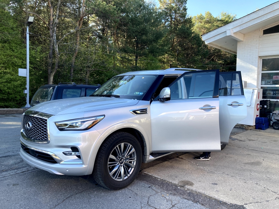 Our ride for the day - a brand new Infiniti QX80! Huge on the outside but suprisingly cramped inside.
 Night Sky at Cherry Springs. The Milky Way galaxy is far more apparent with a camera than it is to the eye.
 Milky Way from the Public Sky Viewing area.
 Tired but happy on the return
03 Apr 2021
I am happy to announce that as of 905am, April 3 2021, I am part of a rapidly increasing COVID19 statistic - the number of people vaccinated from the disease!
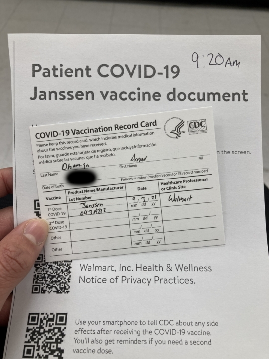 The time in top-right corner of the vaccine document is the time at which I could safely leave after observing a 15 minute waiting period for side effects
I was able to get the Janssen/J&J single dose vaccine a bit earlier than expected by getting a callback from Walmart's leftover vaccine waitlist and I am absolutely delighted to receive this particular vaccine. On the drive back from Walmart, I had Vampire Weekend's Harmony Hall (a song which I had played on repeat for much of 2020) playing on the car's stereo and I felt a surge of positivity that I had been missing for a long time.
I experienced some pretty strong side-effects from the J&J vaccine with chills, a headache, and a fever which reminded me of what bad viral fevers used to feel like after not having gotten sick in over a year. I had an ibuprofen when the symptoms started to get worse and by the next morning, the fever was gone. I was feeling a little weak for most of the day, but otherwise I felt pretty normal. It was definitely the strongest reaction I've ever had to a vaccine, but I have no complaints about it.
I think the biggest positive impact on being fully vaccinated in two weeks will be the added peace of mind in knowing that social decisions can be made with without the mental gymnastics we all used to think through in 2020. It might take a little longer for things to really open back up in the US, but till then, this vaccine will make the ride a lot smoother. Vaccines for my demographic and area are still hard to come by, but fortunately it looks like that will change quickly in the next few weeks when general eligibility opens.