Introduction to Model Predictive Control
Model Predictive Control (MPC) is an incredibly powerful technique for computer aided control of a system. MPC is now used in areas such as aircraft autopilot, traction control in cars, and even HVAC systems to reduce energy costs. In robotics, MPC plays an important role in trajectory generation and path following applications. That said, MPC found its roots in the 1980s in an entirely different type of industry - chemical and oil refinery. Back in those days, compute power was scarce and expensive. By applying an MPC control scheme to the plant’s control systems, operators could save a lot of money which more than justified the cost of using expensive computers. Over time, with increases in compute power and efficiency, it became feasible to run optimization routines for realtime applications.
Before learning about MPC, I only knew about PID control and like PID, MPC is also a closed loop control scheme where the input chosen at a particular time depends on the current state of the system.
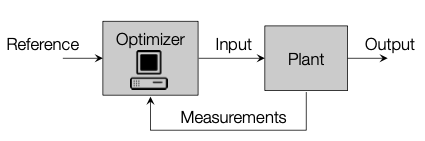 Block diagram of MPC, stolen from Prof. Morari’s lecture slides
While PID can work reasonably well without any knowledge of the system we’re controlling, MPC needs a model of the system we are working with. The benefit of using MPC is that we can obtain an optimal series of inputs if we implement our controller correctly. We can even define what optimal means depending on our application. For instance, for an autonomous drone, an optimal trajectory may be one that minimizes the energy used. On the other hand, for a robotic manipulator, we might want to optimize for minimizing the deviation from a planned trajectory.
One of my favorite parts of MPC is that the theory delves into a number of diverse topics such as control theory, convex optimization, and even computational geometry. With this blog post, I want to give an introduction to MPC and some of its associated concepts.
Discrete Systems
Most practical MPC implementations work with linear, discrete time systems. As the name implies, these are represented with a linear equation as:
\[x_{t+1}=Ax_t+Bu_t\]where $x_t$ represents the state of the system, $A$ is the state transition matrix, $B$ is the input matrix, and $u_t$ is the input. $\Delta_t$ refers to the time discretization of our system. As an example, if we have a drone with a flight computer which can control the motors and sense the drone’s state at 10Hz, we would want to set $\Delta_t$ to 0.1s. Our choice of state $x_t$ in this case is vector representing roll, pitch, and yaw, and our control input $u_t$ can be a vector of throttle inputs to the drone’s motors.
What the above equation is telling us is that given the current state and control input of our system, we can calculate the state of the system at the next timestep. This is the model of the system which helps us predict the future states in our control scheme.
This simple equation is surprisingly powerful and it can be used to represent many different types of control systems. We can even represent systems with non-linear functions (such as sine, cosine, etc.) in their state transition matrix by linearizing the function at each timestep about an operating point.
This explanation is incomplete without an example and I suggest taking a look here for one. Although the system in the example is a continuous time system, discrete time system equations (mostly!) work the same way. The main difference between the continuous system in the example and discrete time systems we are dealing with here is that continuous systems calculate the rate of the system, whereas discrete time systems calculate the next state given the current state.
Cost Function
There are many ways to formulate an MPC problem, but the one we’re going to look at here is picking a series of $n$ control inputs $u_0, u_1,..,u_{n-1}$ to stabilize a system to equilibrium. This means that by applying these $n$ inputs one after the other, we should be able to make the state of the system result in all zeroes at the end.
To use an optimizer based approach for finding an optimal solution, we need a cost function to evaluate the current state. We may also want to be economical with the amount of input applied, so we can assign a cost for the input applied too.
The choice of cost function is based on our problem and there are often different options we can choose to minimize. That said, we would ideally want to pick a cost function which can be optimized easily with the optimization tools we have at hand. For many practical problems, a quadratic cost function is a great choice. This cost function is convex, which guarantees we will find a globally optimal solution if it exists! Moreover, there are open-source implementations of quadratic program solvers such as OSQP. MATLAB’s quadprog works well for these problems too. With a quadratic cost function, and a constraint on our input* our cost may look like this for a single timestep:
In this we can see that $x_t^TQx_t$ is the cost of the state of the system. If $Q$ is positive definite, any non-zero state will have a positive cost. If the system is at equilibrium, the cost will be 0. We can also intuitively see from the equation that if the L2 norm of the state is larger, the cost of the state will be roughly larger as well. Similarly, the term $u_t^TRu_t$ assigns a higher cost for larger inputs.
We can pick a diagonal matrix $Q\geq0$, and scalar $R\gt0$ so our cost is positive if we’re not at equilibrium. We also enforce $\pm u \leq 1$ for the input constraint.
First, let’s (quite charitably) assume we have all the time in the world to stabilize our system. We can then keep picking inputs at each timestep until our system is stable. If we have infinite time, we need to pick a series of infinite inputs! So our overall cost for the entire series ends up looking like:
\[\sum^{\infty}_{t=0} x_t^TQx_t+u_t^TRu_t\]Fortunately, the above sum is not actually infinite, as once we have driven the system to stability, we don’t need to apply any more inputs if the system is stabilizable. All the terms in the above are known because of the recurrence relation we know from the model of the system. But its clearly infeasible to optimize over an infinite series of states and inputs, and this brings us to the next innovation in MPC.
*If we didn’t have any constraints in this optimization problem, an LQR controller would’ve given us a closed form optimal solution by solving the Discrete Algebraic Ricatti Equation (DARE, isn’t this a cool acronym?).
Finite Horizon
Based on sound mathematical arguments which I won’t discuss here, we don’t actually need to compute the solution for infinite states. Instead, we can set a time horizon of a finite number of future $N$ states. This reduces our optimization problem to:
\[\text{minimize } \sum^{N-1}_{t=0} x_t^TQx_t+u_t^TRu_t+x_N^TPx_N\\ \text{subject to } x_{t+1}=Ax_t+Bu_t \text{ and} \pm u \leq 1\]The last term $x_N^TPx_N$ tacked on to the summation is terminal cost which is our estimate for what the remaining cost till infinity will be. This is key here, we are trying to approximate an infinite sum with a reasonable guess for what the infinite sum should be. The choice of the positive definite matrix $P$ is also upto us, but it typically has larger eigenvalues than $Q$. The terminal state also needs to belong to a terminal set which can be calculated using other techniques based on our model.
We will get inputs $u_1,u_2,…,u_{N-1}$ from plugging the above summation into our optimizer of choice. Now, we come to the control part of MPC! We will only use the first input and discard the rest! This sounded wasteful to me when I was first learning about MPC, but the reasoning behind this is that inputs after $u_1$ are calculated based on future states based on our assumed model of the system. In other words, the input $u_2$ we will apply after applying $u_1$ assumes that we would have perfectly reached $x_2=Ax_1+Bu_1$. However, this is based on our model for the system’s dynamics. In the real world, there will be differences in the state we get after applying $u_1$ because of noise, potential linearization error, state estimation error, and errors in our assumption of what the system’s model is to begin with. From a closed loop control perspective, it also makes more sense to only apply the input corresponding to our current state.
Once we have applied $u_1$, we repeat the optimization procedure after measuring our state after applying this input. Just as with the other parameters we have discussed before, the length of the finite time horizon depends on our problem. Too short and it won’t be optimizing over enough states to give us an optimal solution. Too large and our quadratic program might take too long for solve for the hardware we have at hand. On that note, we would ideally want the upper bound of the MPC procedure’s runtime to be the length of one timestep $\Delta_t$. That way, we will have the solution ready before we apply the next input.
Matrix Construction
Quadratic program solvers take a cost function in the form of a single matrix $H$, which is internally used to evaluate $X^THX$ with (optional) constraints on the states. This means we have to rewrite our summation above in the form of a single vector representing all the variables in our optimization. There are two main ways we can do this:
- QP by substitution: replace all the states $x_1…x_n$ by inputs by applying the substitution $x_{t+1}=Ax_t+Bu_t$ everywhere. Optimize only over the inputs.
- QP without substitution: use the equation $x_{t+1}=Ax_t+Bu_t$ as an equality constraint and optimize over both states and inputs. This increases our optimization variables, but this method is actually more computationally efficient than using substitution.
More about these methods can be found from slide 33 onwards here.
While out of scope of this article, there are even ways to find closed form solutions to the MPC problem! A closed form solution can save us from running a computationally intensive optimization routine every timestep. This method deserves an article of its own and it has many benefits in real world applications. We can use this to compute the closed form solution offline and then evaluate the solution using these equations on the target hardware which may not be powerful enough to run the optimization procedure in real time.
To Sum Up
MPC is a valuable tool and we have several ‘hyperparameters’ we can play with like the cost matrices, length of time horizon, and the cost function itself. Finding a good set of parameters requires trial and error based on how our system actually behaves on running on our controller. This post only scratches the surface of MPC, so if you want to learn more about predictive control in all its glory, check out the links in the references section!
References
- https://www.itk.ntnu.no/fag/fordypning/TK16-filer/Samling1_MorariLee.pdf
- https://engineering.utsa.edu/ataha/wp-content/uploads/sites/38/2017/10/MPC_Intro.pdf
- https://www.uiam.sk/pc11/data/workshops/mpc/MPC_PC11_Lecture1.pdf
- http://underactuated.mit.edu/lqr.html
- https://www.ni.com/en-in/innovations/white-papers/06/pid-theory-explained.html
- http://cse.lab.imtlucca.it/~bemporad/teaching/mpc/stuttgart_2012/5-hybrid_mpc.pdf